How did Australia do in the PISA study

Introduction

The purpose of this article is to explore some of the variables that influenced Australia’s performance in PISA study. Note that this is an observational study (as oppose to controlled experiment), and we are inferring on factors that are correlated with academic performance rather than specific causes.

Loading the packages and data

#loading the data and libraries
library(learningtower)
library(tidyverse)
library(lme4)
library(ggfortify)
library(sjPlot)
library(patchwork)
library(ggrepel)
library(kableExtra)

student <- load_student("all")
data(countrycode)

theme_set(theme_classic(18) 
          + theme(legend.position = "bottom"))

Visualise predictors over time

Since we are expecting some time variations in the data, let’s quickly visualize the time trends.

#filtering the data for Australia
aus_data = student %>% 
  dplyr::filter(country %in% c("AUS")) %>% 
  dplyr::mutate(mother_educ = mother_educ %>% fct_relevel("less than ISCED1"),
    father_educ = father_educ %>% fct_relevel("less than ISCED1"))

Numeric variables

A boxplot is a standardized method of presenting data distribution. It informs whether or not our data is symmetrical. Box plots are important because they give a visual overview of the data, allowing researchers to rapidly discover mean values, data set dispersion, and skewness. In this data we visualize the numeric distribution across the years via boxplots.

# plotting the distribution of numeric variables via boxplots
aus_data %>% 
  select(where(is.numeric)) %>% 
  bind_cols(aus_data %>% select(year)) %>% 
  pivot_longer(cols = -year) %>% 
  ggplot(aes(x = year, y = value,
             colour = year)) +
  geom_boxplot() +
  facet_wrap(~name, scales = "free_y") +
  theme(legend.position = "none") +
  labs(x = "Year", 
       y = "", 
       title = "The distribution of numerical variables in the student dataset over all years")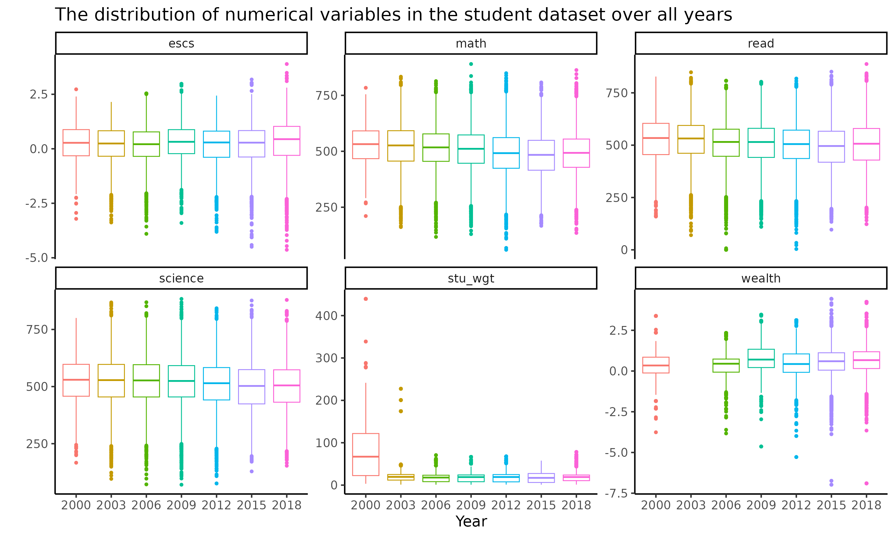

Factor variables

Missing data is a common issue that data professionals must deal with on a daily basis. In this section we visualize the number of missing values across the years for all the factor variables in the student dataset.

#checking the missing values in the factor variables of the data
aus_fct_plotdata = aus_data %>% 
  select(where(is.factor)) %>% 
  dplyr::select(-country, -school_id, -student_id) %>% 
  pivot_longer(cols = -year) %>% 
  group_by(year, name, value) %>% 
  tally() %>% 
  dplyr::mutate(
    value = coalesce(value, "missing"),
    percent = n/sum(n),
    year = year %>% as.character() %>% as.integer()) %>% 
  group_by(name, value) %>% 
  dplyr::mutate(last_point = ifelse(year == max(year), as.character(value), NA))

aus_fct_plotdata %>% 
  ggplot(aes(x = year, y = percent,
             label = last_point,
             group = value)) +
  geom_point() + 
  geom_line() +
  geom_label_repel(direction = "both", nudge_x = 3, seed = 2020, segment.size = 0) +
  facet_wrap(~name, scales = "free_y", ncol = 3) +
  scale_x_continuous(breaks = c(2000, 2003, 2006, 2009, 2012, 2015, 2018)) +
  scale_y_continuous(labels = scales::percent) +
  labs(x = "Year", 
       y = "Percentage of missing values",
       title = "Missing values in the student dataset's factor variables")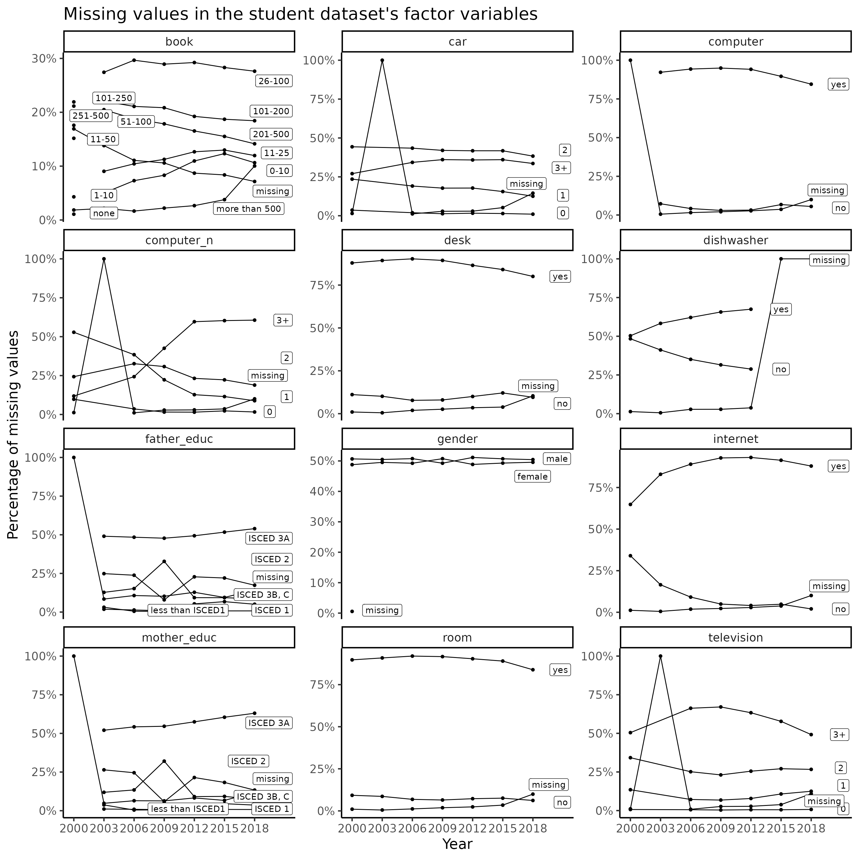

We initially investigate the most current 2018 data before generalizing the models/results into any patterns due to the quantity of missing values in the data in previous years and also to decrease the time complexity in modeling.

Linear regression model for the 2018 study

Linear regression analysis predicts the value of one variable depending on the value of other variables. Because they are well known and can be trained rapidly, linear regression models have become a effective way of scientifically and consistently predicting the future.

We begin by doing a basic data exploration using linear regression models. To begin, we fit three linear models (one for each subject of math, reading, and science) to the 2018 Australian data to gain an understanding of the key variables that may be impacting test scores.

We filter the student data (we use the complete student data obtained by the load student(“all”) function) to pick the scores in Australia and re level some variables for further analyses.

#filtering the data to Australia, defining the predictors and selecting the scores
student_predictors = c("mother_educ", "father_educ", "gender", "internet", 
                       "desk", "room", "television", "computer_n", 
                       "car", "book", "wealth", "escs")

student_formula_rhs = paste(student_predictors, collapse = "+")

aus2018 = aus_data %>% 
  filter(year == "2018") %>% 
  dplyr::select(
    math, read, science, 
    all_of(student_predictors)) %>% 
  na.omit()

Checking correlation matrix of the numeric variables

A correlation matrix is a table that displays the coefficients of correlation between variables. Each cell in the table represents the relationship between two variables.

#correlation matrix for the numeric variables
aus2018 %>% 
  select(where(is.numeric)) %>% 
  cor(use = "pairwise.complete.obs") %>% 
  round(2) %>% 
  kbl(caption = "Correlation Matrix") %>% 
  kable_styling(full_width = NULL,
                position = "center",
                bootstrap_options = c("hover", "striped"))

Correlation Matrix
	math	read	science	wealth	escs
math	1.00	0.78	0.84	0.07	0.33
read	0.78	1.00	0.84	0.03	0.32
science	0.84	0.84	1.00	0.03	0.31
wealth	0.07	0.03	0.03	1.00	0.47
escs	0.33	0.32	0.31	0.47	1.00

Fitting three linear models

#fitting linear models for the three subjects maths, reading and science

aus2018_math = lm(formula = as.formula(paste("math ~ ", student_formula_rhs)) , data = aus2018)

aus2018_read = lm(formula = as.formula(paste("read ~ ", student_formula_rhs)) , data = aus2018)

aus2018_science = lm(formula = as.formula(paste("science ~ ", student_formula_rhs)) , data = aus2018)

sjPlot::tab_model(aus2018_math, aus2018_read, aus2018_science,
                  show.ci = FALSE, show.aic = TRUE, show.se = TRUE,
                  show.stat = TRUE,
                  show.obs = FALSE)

	math				read				science
Predictors	Estimates	std. Error	Statistic	p	Estimates	std. Error	Statistic	p	Estimates	std. Error	Statistic	p
(Intercept)	330.18	16.51	20.00	<0.001	280.37	18.97	14.78	<0.001	318.64	18.14	17.57	<0.001
mother educ [ISCED 1]	2.32	10.19	0.23	0.820	8.95	11.71	0.76	0.445	5.81	11.20	0.52	0.604
mother educ [ISCED 2]	2.09	9.73	0.22	0.830	13.32	11.18	1.19	0.234	7.28	10.69	0.68	0.496
mother educ [ISCED 3A]	11.16	9.64	1.16	0.247	19.23	11.07	1.74	0.083	12.30	10.59	1.16	0.245
mother educ [ISCED 3B, C]	-1.86	9.92	-0.19	0.851	4.58	11.40	0.40	0.688	-1.63	10.90	-0.15	0.881
father educ [ISCED 1]	29.39	9.70	3.03	0.002	28.79	11.15	2.58	0.010	10.65	10.66	1.00	0.318
father educ [ISCED 2]	15.71	9.42	1.67	0.095	23.47	10.82	2.17	0.030	20.42	10.34	1.97	0.048
father educ [ISCED 3A]	33.76	9.38	3.60	<0.001	39.37	10.78	3.65	<0.001	32.32	10.31	3.14	0.002
father educ [ISCED 3B, C]	21.18	9.61	2.20	0.028	29.69	11.05	2.69	0.007	22.12	10.56	2.09	0.036
gender [male]	10.14	1.59	6.40	<0.001	-24.94	1.82	-13.69	<0.001	9.69	1.74	5.56	<0.001
internet [yes]	33.83	6.06	5.58	<0.001	38.44	6.97	5.52	<0.001	35.63	6.66	5.35	<0.001
desk [yes]	16.69	2.76	6.05	<0.001	17.39	3.17	5.49	<0.001	15.96	3.03	5.27	<0.001
room [yes]	9.05	3.23	2.80	0.005	4.95	3.72	1.33	0.183	4.35	3.55	1.22	0.221
television [1]	19.18	8.95	2.14	0.032	29.02	10.29	2.82	0.005	24.39	9.84	2.48	0.013
television [2]	9.83	8.90	1.10	0.269	27.33	10.23	2.67	0.008	21.53	9.78	2.20	0.028
television [3+]	-3.70	8.96	-0.41	0.680	15.37	10.30	1.49	0.136	5.26	9.85	0.53	0.594
computer n [1]	-7.33	7.41	-0.99	0.322	9.07	8.51	1.07	0.287	-1.17	8.14	-0.14	0.886
computer n [2]	16.39	7.33	2.24	0.025	36.30	8.42	4.31	<0.001	25.57	8.05	3.18	0.001
computer n [3+]	36.64	7.44	4.92	<0.001	55.45	8.55	6.48	<0.001	37.14	8.18	4.54	<0.001
car [1]	6.69	8.41	0.80	0.426	26.09	9.66	2.70	0.007	12.68	9.24	1.37	0.170
car [2]	15.90	8.40	1.89	0.058	34.54	9.66	3.58	<0.001	19.75	9.23	2.14	0.032
car [3+]	6.93	8.56	0.81	0.418	22.60	9.84	2.30	0.022	9.19	9.41	0.98	0.328
book101-200	34.36	3.11	11.03	<0.001	58.51	3.58	16.34	<0.001	53.46	3.42	15.62	<0.001
book11-25	10.24	3.25	3.15	0.002	12.32	3.74	3.29	0.001	6.75	3.58	1.89	0.059
book201-500	48.97	3.32	14.73	<0.001	74.83	3.82	19.59	<0.001	69.20	3.65	18.95	<0.001
book26-100	31.12	2.87	10.83	<0.001	45.04	3.30	13.64	<0.001	40.73	3.16	12.90	<0.001
book [more than 500]	33.30	3.89	8.57	<0.001	66.07	4.47	14.79	<0.001	60.88	4.27	14.26	<0.001
wealth	-12.57	1.61	-7.80	<0.001	-21.05	1.85	-11.37	<0.001	-15.44	1.77	-8.72	<0.001
escs	18.05	1.37	13.14	<0.001	20.15	1.58	12.77	<0.001	17.05	1.51	11.30	<0.001
R² / R² adjusted	0.196 / 0.194				0.223 / 0.221				0.192 / 0.190
AIC	129529.762				132618.597				131619.367

Some interesting discoveries from these models:

All three response variables seem to be influenced by the same set of factors.
Father’s education level (father_educ) seems to have a much stronger effect than mother’s education level (mother_educ).
While most estimates agree in signs across the three subjects, the most notable exception to this is gender, where girls tend to perform better than boys in reading.
The most influential predictors are those associated with socioeconomic status (escs) and education (book). A number of variables that should not be directly causal to academic performance also showed up as significant. This is likely due to their associations with socio-economic status.

Upon checking the classical diagnostic plots of these models, we see no major violation on the assumptions of linear models. The large amount of variations in the data may help to explain why the models only has a moderately low \(R^2\) values (~ 0.20).

#plotting the outcome of linear models
autoplot(aus2018_math) + labs(title = "2018 Australia maths model") +
autoplot(aus2018_read) + labs(title = "2018 Australia read model") + 
autoplot(aus2018_science) + labs(title = "2018 Australia science model")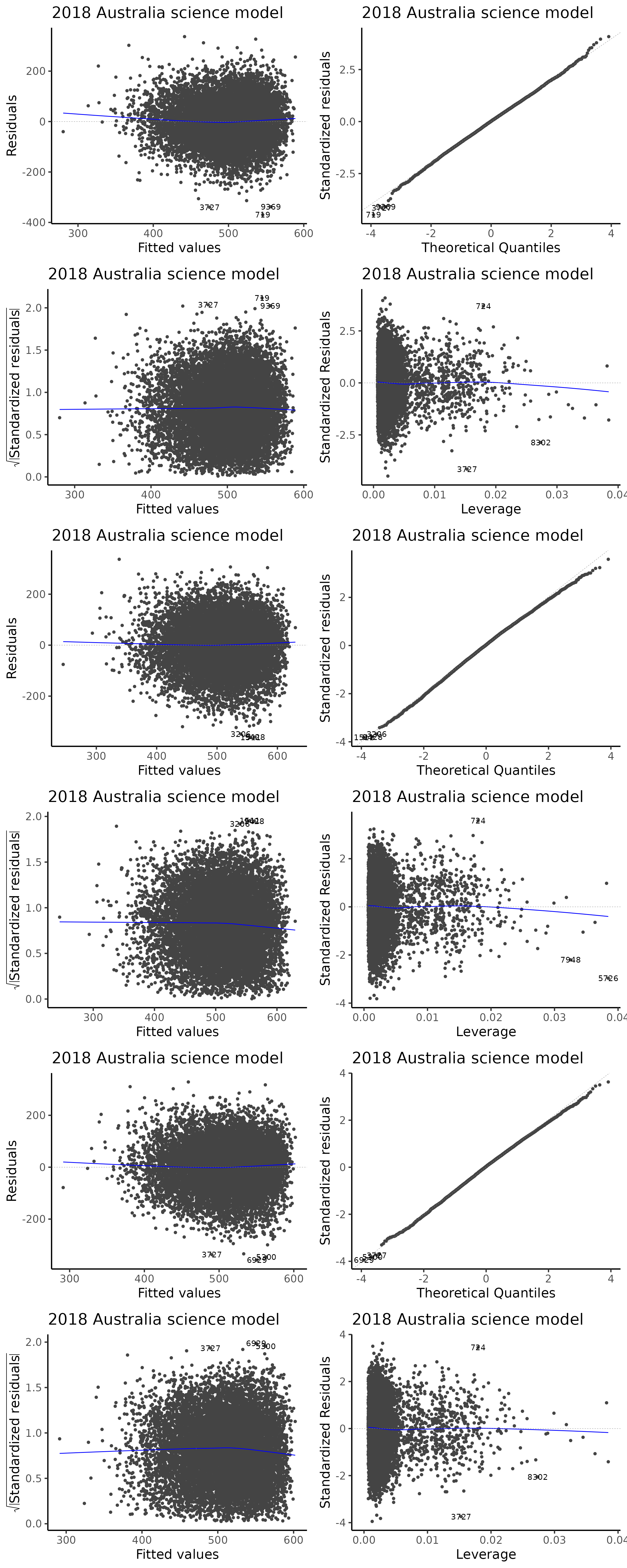

Linear mixed model

Linear mixed models are a subset of simple linear models that allow for both fixed and random effects.

We already know that the socio-economic status (SES) of a student is often the most influential predictor and it is likely that students with similar SES will attend the same schools in their neighborhood and receive similar level of quality of education from the same teachers.

Thus, it is likely that there will be a grouping effect on the students if they attended the same school. This would imply that some observations in our data are not independent observations.

By building random effects in our linear model, that is building a linear mixed model, we should be able to produce a model with better fit if we consider this grouping effect of schools into our model.

# joining school and student data, building a linear mixed model
lmm2018 = aus_data %>% 
  filter(year == "2018") %>% 
  select(
    school_id,
    math, read, science, 
    all_of(student_predictors)) %>% 
  na.omit()

lmm2018_math = lmer(formula = as.formula(paste("math ~ ", student_formula_rhs, "+ (escs | school_id)")), data = lmm2018)

lmm2018_read = lmer(formula = as.formula(paste("read ~ ", student_formula_rhs, "+ (escs | school_id)")), data = lmm2018)

lmm2018_science = lmer(formula = as.formula(paste("science ~ ", student_formula_rhs, "+ (escs | school_id)")), data = lmm2018)

sjPlot::tab_model(lmm2018_math, lmm2018_read, lmm2018_science,
                  show.ci = FALSE, show.aic = TRUE, show.se = TRUE,
                  show.stat = TRUE,
                  show.obs = FALSE)

	math				read				science
Predictors	Estimates	std. Error	Statistic	p	Estimates	std. Error	Statistic	p	Estimates	std. Error	Statistic	p
(Intercept)	317.19	16.19	19.59	<0.001	266.75	18.94	14.08	<0.001	304.84	17.84	17.09	<0.001
mother educ [ISCED 1]	7.61	9.82	0.78	0.438	14.29	11.52	1.24	0.215	12.98	10.84	1.20	0.231
mother educ [ISCED 2]	10.68	9.40	1.14	0.256	21.22	11.03	1.92	0.054	16.21	10.38	1.56	0.118
mother educ [ISCED 3A]	18.21	9.30	1.96	0.050	25.87	10.91	2.37	0.018	19.81	10.27	1.93	0.054
mother educ [ISCED 3B, C]	8.24	9.57	0.86	0.389	13.83	11.23	1.23	0.218	9.00	10.57	0.85	0.394
father educ [ISCED 1]	32.51	9.37	3.47	0.001	31.61	10.99	2.88	0.004	13.03	10.34	1.26	0.208
father educ [ISCED 2]	19.96	9.09	2.20	0.028	27.17	10.66	2.55	0.011	23.40	10.03	2.33	0.020
father educ [ISCED 3A]	33.61	9.06	3.71	<0.001	39.91	10.62	3.76	<0.001	31.94	9.99	3.20	0.001
father educ [ISCED 3B, C]	25.74	9.28	2.77	0.006	33.08	10.88	3.04	0.002	25.04	10.24	2.45	0.014
gender [male]	9.18	1.60	5.72	<0.001	-24.99	1.87	-13.39	<0.001	9.07	1.77	5.12	<0.001
internet [yes]	32.45	5.82	5.58	<0.001	37.57	6.83	5.50	<0.001	34.95	6.44	5.43	<0.001
desk [yes]	15.48	2.63	5.88	<0.001	17.09	3.09	5.53	<0.001	15.08	2.91	5.18	<0.001
room [yes]	8.17	3.11	2.62	0.009	4.11	3.65	1.13	0.260	3.53	3.45	1.02	0.306
television [1]	18.13	8.85	2.05	0.040	30.01	10.30	2.91	0.004	26.04	9.77	2.67	0.008
television [2]	11.70	8.81	1.33	0.184	29.95	10.25	2.92	0.003	25.34	9.73	2.61	0.009
television [3+]	2.05	8.88	0.23	0.818	21.04	10.33	2.04	0.042	12.87	9.80	1.31	0.189
computer n [1]	-3.56	7.12	-0.50	0.617	12.52	8.36	1.50	0.134	2.16	7.87	0.27	0.784
computer n [2]	20.74	7.07	2.93	0.003	40.11	8.30	4.83	<0.001	28.73	7.81	3.68	<0.001
computer n [3+]	40.27	7.19	5.60	<0.001	59.13	8.44	7.01	<0.001	40.24	7.95	5.06	<0.001
car [1]	7.71	8.08	0.95	0.340	26.48	9.48	2.79	0.005	12.85	8.93	1.44	0.150
car [2]	16.44	8.08	2.03	0.042	34.50	9.48	3.64	<0.001	19.40	8.93	2.17	0.030
car [3+]	11.50	8.25	1.39	0.163	25.58	9.67	2.64	0.008	12.05	9.12	1.32	0.186
book101-200	31.59	3.00	10.54	<0.001	55.33	3.51	15.76	<0.001	50.09	3.32	15.11	<0.001
book11-25	10.12	3.11	3.25	0.001	12.01	3.65	3.29	0.001	6.77	3.45	1.97	0.049
book201-500	44.39	3.20	13.88	<0.001	70.78	3.75	18.89	<0.001	64.62	3.54	18.27	<0.001
book26-100	29.19	2.76	10.58	<0.001	43.13	3.23	13.34	<0.001	39.00	3.05	12.78	<0.001
book [more than 500]	32.41	3.76	8.62	<0.001	65.30	4.40	14.85	<0.001	60.08	4.15	14.46	<0.001
wealth	-14.85	1.57	-9.45	<0.001	-23.34	1.84	-12.71	<0.001	-18.08	1.73	-10.42	<0.001
escs	13.12	1.41	9.29	<0.001	16.26	1.63	9.95	<0.001	12.74	1.54	8.29	<0.001
Random Effects
σ²	5898.15				8154.47				7239.62
τ₀₀	732.06 _{school_id}				718.60 _{school_id}				858.93 _{school_id}
τ₁₁	133.29 _{school_id.escs}				145.17 _{school_id.escs}				110.18 _{school_id.escs}
ρ₀₁	0.36 _{school_id}				0.18 _{school_id}				0.30 _{school_id}
ICC	0.14				0.10				0.12
N	732 _{school_id}				732 _{school_id}				732 _{school_id}
Marginal R² / Conditional R²	0.144 / 0.262				0.191 / 0.271				0.153 / 0.258
AIC	128734.532				132139.368				130935.163

We see that the linear mixed model improved on the fit of the model, as judged by the AIC.

# subtracting AIC values of the two models
bind_cols(
AIC(aus2018_math) - AIC(lmm2018_math),
AIC(aus2018_read) - AIC(lmm2018_read),
AIC(aus2018_science) - AIC(lmm2018_science)
) %>% 
  rename(maths = ...1,
         read = ...2,
         science = ...3) %>% 
  kbl(caption = "AIC Values") %>% 
  kable_styling(full_width = NULL,
                position = "center",
                bootstrap_options = c("hover", "striped"))

AIC Values
maths	read	science
795.2309	479.2288	684.2047

Integrating with `school` data

We now take this dataset on students and merge it with some variables from the school data which is also a part of this learningtower package. This allows us to gain more access to the school level variables this is helpful in modelling the data.

#taking into account the school dataset variables and fitting a linear mixed model
selected_vars = c("father_educ", "gender", "internet", 
                  "desk", "computer_n", "car",
                  "book", "wealth", "escs")

data(school)

aus_school_2018 = school %>% 
  dplyr::filter(country == "AUS", year == "2018") %>% 
  dplyr::mutate(school_size = log10(school_size)) %>% ## We take the log due to the scale
  dplyr::select(-year, -country, -contains("fund"), -sch_wgt)

lmm2018_sch = lmm2018 %>% 
  left_join(aus_school_2018, by = c("school_id")) %>% na.omit()

school_predictors = c("stratio", "public_private", "staff_shortage", "school_size")
school_formula_rhs = paste(school_predictors, collapse = "+")

lmm2018_sch_math = lmer(formula = as.formula(paste("math ~ ", student_formula_rhs, "+ (escs | school_id) + ",
                                                   school_formula_rhs)), data = lmm2018_sch)

lmm2018_sch_read = lmer(formula = as.formula(paste("read ~ ", student_formula_rhs, "+ (escs | school_id) + ",
                                                   school_formula_rhs)), data = lmm2018_sch)

lmm2018_sch_science = lmer(formula = as.formula(paste("science ~ ", student_formula_rhs, "+ (escs | school_id) + ",
                                                      school_formula_rhs)), data = lmm2018_sch)


sjPlot::tab_model(lmm2018_sch_math, lmm2018_sch_read, lmm2018_sch_science,
                  show.ci = FALSE, show.aic = TRUE, show.se = TRUE,
                  show.stat = TRUE,
                  show.obs = FALSE)

	math				read				science
Predictors	Estimates	std. Error	Statistic	p	Estimates	std. Error	Statistic	p	Estimates	std. Error	Statistic	p
(Intercept)	208.64	23.11	9.03	<0.001	165.01	25.92	6.37	<0.001	212.87	25.15	8.46	<0.001
mother educ [ISCED 1]	11.15	10.79	1.03	0.302	18.11	12.73	1.42	0.155	11.76	11.90	0.99	0.323
mother educ [ISCED 2]	15.32	10.39	1.48	0.140	25.98	12.25	2.12	0.034	17.74	11.45	1.55	0.121
mother educ [ISCED 3A]	21.66	10.28	2.11	0.035	28.74	12.12	2.37	0.018	19.48	11.34	1.72	0.086
mother educ [ISCED 3B, C]	11.72	10.58	1.11	0.268	15.60	12.48	1.25	0.211	8.08	11.67	0.69	0.488
father educ [ISCED 1]	35.65	10.32	3.46	0.001	34.73	12.17	2.85	0.004	17.88	11.37	1.57	0.116
father educ [ISCED 2]	19.44	10.03	1.94	0.053	29.31	11.83	2.48	0.013	26.47	11.06	2.39	0.017
father educ [ISCED 3A]	33.81	10.00	3.38	0.001	40.66	11.79	3.45	0.001	34.36	11.02	3.12	0.002
father educ [ISCED 3B, C]	27.63	10.24	2.70	0.007	37.49	12.07	3.11	0.002	30.63	11.29	2.71	0.007
gender [male]	8.70	1.74	4.99	<0.001	-25.74	2.03	-12.70	<0.001	8.59	1.92	4.47	<0.001
internet [yes]	29.02	6.37	4.55	<0.001	30.57	7.49	4.08	<0.001	28.92	7.04	4.11	<0.001
desk [yes]	14.15	2.89	4.89	<0.001	14.50	3.39	4.27	<0.001	12.08	3.20	3.78	<0.001
room [yes]	3.66	3.37	1.08	0.279	0.99	3.96	0.25	0.803	0.93	3.73	0.25	0.802
television [1]	12.03	9.58	1.26	0.209	24.94	11.12	2.24	0.025	18.96	10.56	1.80	0.073
television [2]	6.11	9.54	0.64	0.522	25.45	11.07	2.30	0.022	18.16	10.51	1.73	0.084
television [3+]	-4.40	9.61	-0.46	0.647	15.28	11.15	1.37	0.170	5.32	10.59	0.50	0.615
computer n [1]	3.70	7.91	0.47	0.640	15.57	9.32	1.67	0.095	4.31	8.73	0.49	0.621
computer n [2]	27.59	7.86	3.51	<0.001	42.63	9.26	4.60	<0.001	31.73	8.67	3.66	<0.001
computer n [3+]	45.46	7.99	5.69	<0.001	60.32	9.41	6.41	<0.001	41.59	8.82	4.72	<0.001
car [1]	11.91	8.59	1.39	0.166	27.03	10.12	2.67	0.008	15.13	9.49	1.59	0.111
car [2]	20.22	8.59	2.36	0.019	36.07	10.10	3.57	<0.001	21.10	9.48	2.23	0.026
car [3+]	16.64	8.77	1.90	0.058	28.29	10.31	2.74	0.006	15.50	9.68	1.60	0.109
book101-200	32.87	3.27	10.05	<0.001	56.25	3.83	14.67	<0.001	51.98	3.61	14.38	<0.001
book11-25	13.70	3.42	4.00	<0.001	14.52	4.02	3.61	<0.001	11.10	3.78	2.94	0.003
book201-500	46.10	3.49	13.22	<0.001	71.34	4.09	17.44	<0.001	66.97	3.86	17.37	<0.001
book26-100	29.81	3.01	9.89	<0.001	42.65	3.54	12.06	<0.001	39.32	3.33	11.80	<0.001
book [more than 500]	35.82	4.10	8.74	<0.001	67.82	4.80	14.12	<0.001	63.68	4.53	14.06	<0.001
wealth	-15.69	1.72	-9.12	<0.001	-23.88	2.01	-11.85	<0.001	-18.64	1.90	-9.81	<0.001
escs	11.88	1.52	7.80	<0.001	15.52	1.79	8.69	<0.001	11.30	1.66	6.80	<0.001
stratio	0.56	0.32	1.75	0.080	0.32	0.31	1.02	0.309	0.17	0.33	0.51	0.609
public private [public]	-12.29	2.94	-4.18	<0.001	-14.20	2.97	-4.78	<0.001	-14.18	3.11	-4.55	<0.001
staff shortage	-4.27	1.56	-2.74	0.006	-3.61	1.59	-2.27	0.023	-4.68	1.66	-2.83	0.005
school size	37.12	5.52	6.73	<0.001	38.97	5.72	6.82	<0.001	36.88	5.89	6.26	<0.001
Random Effects
σ²	5936.00				8233.78				7285.06
τ₀₀	602.13 _{school_id}				494.18 _{school_id}				655.09 _{school_id}
τ₁₁	83.58 _{school_id.escs}				118.77 _{school_id.escs}				57.79 _{school_id.escs}
ρ₀₁	0.45 _{school_id}				0.17 _{school_id}				0.44 _{school_id}
ICC	0.11				0.07				0.10
N	608 _{school_id}				608 _{school_id}				608 _{school_id}
Marginal R² / Conditional R²	0.181 / 0.273				0.217 / 0.273				0.181 / 0.260
AIC	108233.116				111106.699				110061.230

We note the following:

The school size (school_size) is a strong predictor for academic performance, implying larger schools tend to do better. This is likely a confounding variable for the urban/rural region of the school which can imply a difference in available funding of school facilities.
Private school tends to better than public schools (note the reference level and the negative coefficient estimate in the variable public_private).
Perhaps surprisingly, the student-teacher ratio (stratio) wasn’t found to be significant but the shortage of staff (staff_shortage) was significant. This would imply that as long as the school is adequately supported by staff, further reduction in the student-teacher ratio does not have a statistical significant effect on student performance.

Visualising coefficient estimates over the years

All analyses above focused on the year 2018 for Australia, but what about the other years? We also visualize the academic performances of students as a function of time in the time trend article, so in this section, we attempt to visualize the effect of some interesting variables and their linear model coefficient estimates for each of the PISA study over time.

We would expect the availability of technology (e.g. computer) could be beneficial for students at the start of the 21st century, but it is not clear if students will be helped by these technologies as time goes by.

The construction goes as follow:

We first split the entire Australian data by year and fit a linear model, with math as the response variable.
We extract the coefficient estimate for every predictor from every linear model and combine the result.
We then plot the years on the x-axis and the coefficient estimates on the y-axis as points and join each variable using a line. For categorical variables, we split the categories as separate lines.
Additionally, we show the 95% confidence interval of each coefficient estimate using a transparent ribbon and show the y = 0 line. i.e. whenever the ribbon crosses the horizontal line, the p-value for testing this level will be < 0.05.

#Fitting a linear model, extracting the coefficients and visualizing every predictor
aus_student_years = aus_data %>% 
  dplyr::select(
    math,
    all_of(student_predictors),
    year) %>% 
  na.omit()

aus_student_years_coef = aus_student_years %>% 
  group_by(year) %>% 
  nest() %>% 
  dplyr::mutate(math_lm_coef = purrr::map(.x = data, 
                              .f = ~ lm(formula = as.formula(paste("math ~ ", student_formula_rhs)), data = .x) %>% 
                                broom::tidy())) %>% 
  dplyr::select(-data) %>% 
  tidyr::unnest(math_lm_coef)

aus_student_years_coef %>% 
  dplyr::filter(str_detect(term, "computer|father_educ|escs|wealth")) %>% 
  dplyr::mutate(
    year = year %>% as.character() %>% as.integer(),
    facet = case_when(
      str_detect(term, "computer") ~ "Number of computer",
      str_detect(term, "father_educ") ~ "Education of father",
      # str_detect(term, "mother_educ") ~ "Education of mother",
      str_detect(term, "wealth") ~ "Wealth",
      str_detect(term, "escs") ~ "Socio-economic index"),
    last_point = ifelse(year == 2018, term, NA)) %>% 
  ggplot(aes(x = year, y = estimate,
             colour = term,
             group = term,
             label = last_point)) +
  geom_hline(yintercept = 0) +
  geom_point(position = position_dodge(width = 0.8), size = 2) +
  geom_line(position = position_dodge(width = 0.8), size = 1.5) +
  geom_linerange(aes(ymin = estimate - 2*std.error,
                     ymax = estimate + 2*std.error),
                 size = 4, alpha = 0.7,
                 position = position_dodge(width = 0.8)) +
  geom_label_repel(direction = "both", nudge_x = 2, seed = 2020, segment.size = 0) +
  scale_x_continuous(limits = c(2005.5, 2022),
                     breaks = c(2006, 2009, 2012, 2015, 2018)) +
  facet_wrap(~facet, scales = "free_y") +
  theme(legend.position = "none") +
  labs(x = "Year",
       y = "Estimate",
       title = "Graphing coefficient estimates throughout time")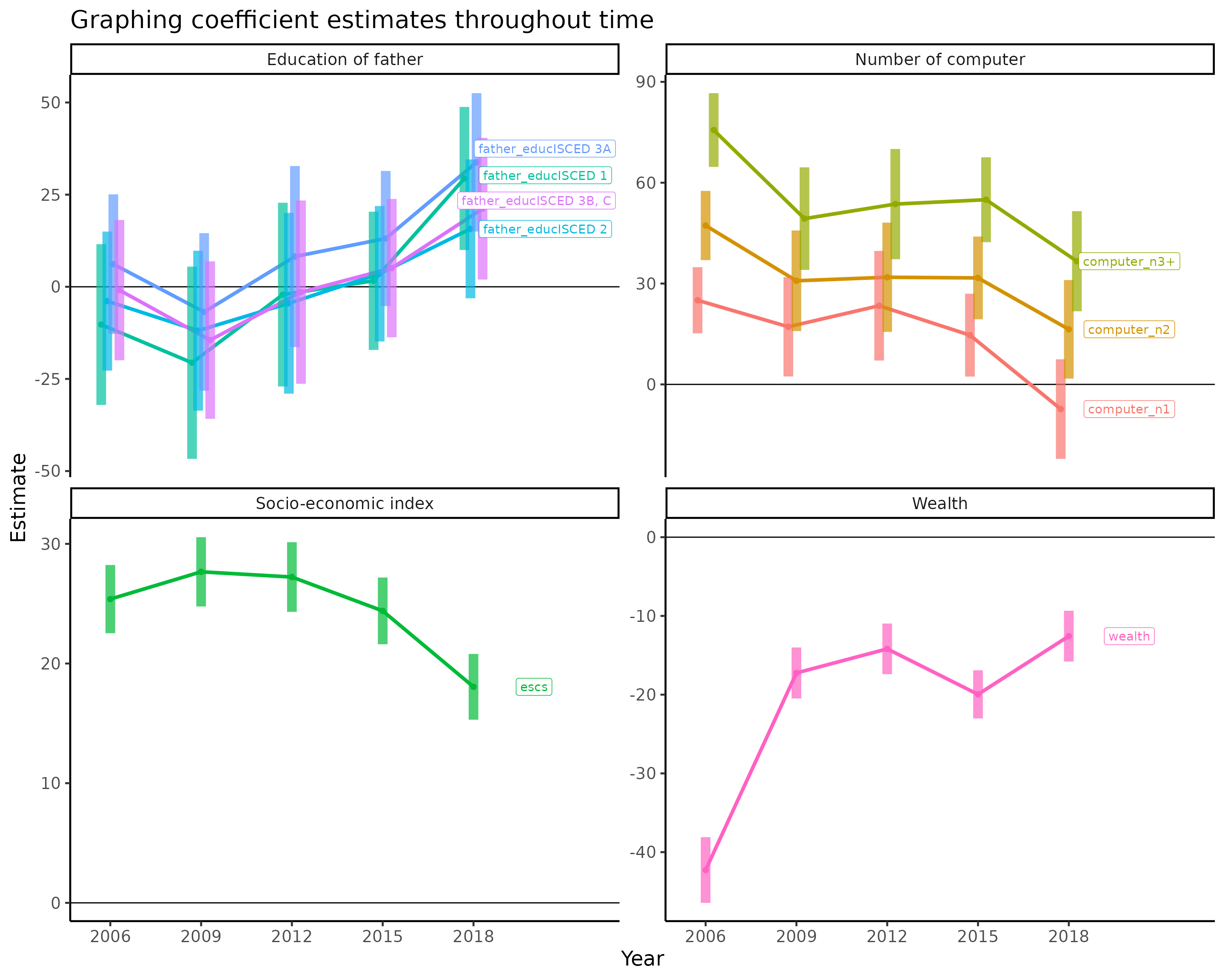

We note the following:

Even though in the 2018, we found the education of father was statistically significant against students’ academic performance, this was not always the case. From 2006 to 2018, the education of father seems to have ever positive influence on students.
It is clear that access to computers is ever more prevalent in Australia. But surprisingly, the positive influence of computers are decreasing. It is not clear why this would be the case. One possible reason is that students might have access to computers outside of their homes (e.g. from schools) and thus the advantages of accessing computers are dampened.
Quite interestingly, the influence of socio-economic index is dropping, implying a gradual move towards equality.

Session info

sessionInfo()
#> R version 4.2.2 (2022-10-31)
#> Platform: x86_64-pc-linux-gnu (64-bit)
#> Running under: Ubuntu 22.04.1 LTS
#> 
#> Matrix products: default
#> BLAS:   /usr/lib/x86_64-linux-gnu/openblas-pthread/libblas.so.3
#> LAPACK: /usr/lib/x86_64-linux-gnu/openblas-pthread/libopenblasp-r0.3.20.so
#> 
#> locale:
#>  [1] LC_CTYPE=C.UTF-8       LC_NUMERIC=C           LC_TIME=C.UTF-8       
#>  [4] LC_COLLATE=C.UTF-8     LC_MONETARY=C.UTF-8    LC_MESSAGES=C.UTF-8   
#>  [7] LC_PAPER=C.UTF-8       LC_NAME=C              LC_ADDRESS=C          
#> [10] LC_TELEPHONE=C         LC_MEASUREMENT=C.UTF-8 LC_IDENTIFICATION=C   
#> 
#> attached base packages:
#> [1] stats     graphics  grDevices utils     datasets  methods   base     
#> 
#> other attached packages:
#>  [1] kableExtra_1.3.4    ggrepel_0.9.3       patchwork_1.1.2    
#>  [4] sjPlot_2.8.12       ggfortify_0.4.15    lme4_1.1-31        
#>  [7] Matrix_1.5-1        forcats_1.0.0       stringr_1.5.0      
#> [10] dplyr_1.1.0         purrr_1.0.1         readr_2.1.4        
#> [13] tidyr_1.3.0         tibble_3.1.8        ggplot2_3.4.1      
#> [16] tidyverse_1.3.2     learningtower_1.0.1
#> 
#> loaded via a namespace (and not attached):
#>  [1] nlme_3.1-160        fs_1.6.1            lubridate_1.9.2    
#>  [4] webshot_0.5.4       insight_0.19.0      httr_1.4.4         
#>  [7] rprojroot_2.0.3     tools_4.2.2         backports_1.4.1    
#> [10] bslib_0.4.2         utf8_1.2.3          R6_2.5.1           
#> [13] sjlabelled_1.2.0    DBI_1.1.3           colorspace_2.1-0   
#> [16] withr_2.5.0         tidyselect_1.2.0    gridExtra_2.3      
#> [19] emmeans_1.8.4-1     curl_5.0.0          compiler_4.2.2     
#> [22] performance_0.10.2  textshaping_0.3.6   cli_3.6.0          
#> [25] rvest_1.0.3         xml2_1.3.3          desc_1.4.2         
#> [28] labeling_0.4.2      bayestestR_0.13.0   sass_0.4.5         
#> [31] scales_1.2.1        mvtnorm_1.1-3       pkgdown_2.0.7      
#> [34] systemfonts_1.0.4   digest_0.6.31       minqa_1.2.5        
#> [37] svglite_2.1.1       rmarkdown_2.20      pkgconfig_2.0.3    
#> [40] htmltools_0.5.4     highr_0.10          dbplyr_2.3.0       
#> [43] fastmap_1.1.0       rlang_1.0.6         readxl_1.4.2       
#> [46] rstudioapi_0.14     farver_2.1.1        jquerylib_0.1.4    
#> [49] generics_0.1.3      jsonlite_1.8.4      googlesheets4_1.0.1
#> [52] magrittr_2.0.3      parameters_0.20.2   Rcpp_1.0.10        
#> [55] munsell_0.5.0       fansi_1.0.4         lifecycle_1.0.3    
#> [58] stringi_1.7.12      yaml_2.3.7          MASS_7.3-58.1      
#> [61] grid_4.2.2          sjmisc_2.8.9        crayon_1.5.2       
#> [64] lattice_0.20-45     ggeffects_1.1.5     haven_2.5.1        
#> [67] splines_4.2.2       sjstats_0.18.2      hms_1.1.2          
#> [70] knitr_1.42          pillar_1.8.1        boot_1.3-28        
#> [73] estimability_1.4.1  effectsize_0.8.3    reprex_2.0.2       
#> [76] glue_1.6.2          evaluate_0.20       modelr_0.1.10      
#> [79] vctrs_0.5.2         nloptr_2.0.3        tzdb_0.3.0         
#> [82] cellranger_1.1.0    gtable_0.3.1        datawizard_0.6.5   
#> [85] assertthat_0.2.1    cachem_1.0.6        xfun_0.37          
#> [88] broom_1.0.3         viridisLite_0.4.1   ragg_1.2.5         
#> [91] googledrive_2.0.0   gargle_1.3.0        memoise_2.0.1      
#> [94] timechange_0.2.0    ellipsis_0.3.2

The Freemasons

2023-02-18

Introduction

Loading the packages and data

Visualise predictors over time

Numeric variables

Factor variables

Linear regression model for the 2018 study

Checking correlation matrix of the numeric variables

Fitting three linear models

Linear mixed model

Integrating with `school` data

Visualising coefficient estimates over the years

Session info

How did Australia do in the PISA study

The Freemasons

2023-02-18

Introduction

Loading the packages and data

Visualise predictors over time

Numeric variables

Factor variables

Linear regression model for the 2018 study

Checking correlation matrix of the numeric variables

Fitting three linear models

Linear mixed model

Integrating with school data

Visualising coefficient estimates over the years

Session info

Integrating with `school` data