Using the Student and Country Data
Source:vignettes/learningtower_student.Rmd
learningtower_student.RmdIntroduction
The goal of learningtower is to provide a user-friendly
R package to provide easy access to a subset of variables from PISA data
collected from the OECD.
Version 1.1.1 of this package provides the data for the years 2000 -
2022. The survey data is published every three years. This is an
excellent real world dataset for data exploring, data visualizing and
statistical computations.
This vignette documents how to access the data, and shows a few typical methods to explore the data.
Exploring the student data
Usage of the subset of the student data
In
learningtower, the main data is the student data. This data contains information regarding student test scores and some selected variables regarding their schooling and socio-economic status. The original and complete data may be obtained from OECD.However, the size of the full
studentis too big to fit inside the package. Hence, in our package, we provide a random subset of the student data, stored asstudent_subset_20xxdata objects (wherexxdenotes the specific year of the study). These subset data can be used to understanding the data structure before using the full dataset which is available for download.The student subset data is constructed by randomly sampling from the full student data. For each year and each country, we randomly sample approximately 50 observations.
The complete student dataset is available for download and can be loaded using the
load_student()function included in this package.
Below is a quick example of loading the 2018 subset student data.
library(dplyr)
library(ggplot2)
library(learningtower)

#load the subset student data for the year 2018
data(student_subset_2018)
#load the countrycode data
data(countrycode)

glimpse(student_subset_2018)
#> Rows: 1,900
#> Columns: 22
#> $ year        <int> 2018, 2018, 2018, 2018, 2018, 2018, 2018, 2018, 2018, 2018…
#> $ country     <fct> AUS, AUS, AUS, AUS, AUS, AUS, AUS, AUS, AUS, AUS, AUS, AUS…
#> $ school_id   <chr> "3600310", "3600251", "3600639", "3600704", "3600736", "36…
#> $ student_id  <int> 3606824, 3605794, 3613122, 3611607, 3606403, 3621081, 3611…
#> $ mother_educ <fct> "ISCED 3A", "ISCED 2", "ISCED 3A", "ISCED 3A", NA, "ISCED …
#> $ father_educ <fct> "ISCED 3A", "ISCED 1", "ISCED 3A", "ISCED 1", NA, "ISCED 3…
#> $ gender      <fct> male, female, female, female, male, female, male, female, …
#> $ computer    <fct> yes, yes, yes, no, yes, yes, yes, yes, yes, yes, yes, yes,…
#> $ internet    <fct> yes, yes, yes, yes, no, yes, yes, yes, yes, yes, yes, yes,…
#> $ math        <dbl> 427.631, 479.464, 490.057, 517.379, 527.985, 462.708, 307.…
#> $ read        <dbl> 425.307, 513.694, 593.488, 588.042, 535.348, 401.866, 258.…
#> $ science     <dbl> 369.288, 486.794, 469.697, 584.995, 560.943, 467.130, 325.…
#> $ stu_wgt     <dbl> 3.11283, 27.41035, 14.56053, 21.68163, 15.57013, 10.96668,…
#> $ desk        <fct> yes, yes, yes, yes, yes, yes, yes, yes, yes, yes, yes, yes…
#> $ room        <fct> yes, yes, yes, yes, yes, yes, yes, yes, no, yes, yes, yes,…
#> $ dishwasher  <fct> NA, NA, NA, NA, NA, NA, NA, NA, NA, NA, NA, NA, NA, NA, NA…
#> $ television  <fct> 1, 3+, 3+, 2, 2, 3+, 2, 3+, 3+, 3+, 3+, 3+, 2, 1, NA, 2, 1…
#> $ computer_n  <fct> 2, 1, 3+, 1, 3+, 3+, 3+, 3+, 3+, 2, 3+, 1, 3+, 3+, NA, 3+,…
#> $ car         <fct> 3+, 3+, 3+, 3+, 2, 3+, 2, 2, 1, 3+, 3+, 2, 2, 2, NA, 3+, 1…
#> $ book        <fct> 201-500, 101-200, 0-10, 0-10, 26-100, 201-500, 101-200, 26…
#> $ wealth      <dbl> 0.1688, 0.6327, 1.4097, -0.1318, 0.2886, 1.8571, 0.9773, 0…
#> $ escs        <dbl> 1.2100, -0.8160, 0.0932, -0.4153, NA, 0.7428, 0.2569, -0.6…
selected_countries = c("AUS", "USA", "TUR", "SWE",
                       "CHE", "NZL", "BEL", "DEU")

student_subset_2018 |>
  group_by(country, gender) |>
  dplyr::filter(country %in% selected_countries) |>
  dplyr::left_join(countrycode, by = "country") |>
  ggplot(aes(x = math,
             y = country_name,
             fill = gender)) +
  geom_boxplot() +
  scale_fill_manual(values = c("#FF7F0EFF", "#1F77B4FF")) +
  theme_classic() +
  labs(x = "Math score",
       y = "")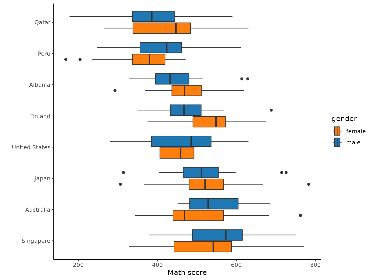
In the figure above, we see that from the student subset data for the year 2018, in the countries like USA and Belgium boys perform better as compared to the girls. However, in countries such as Turkey and Switzerland, girls perform better than the boys or are on the same level with boys when it comes to their average mathematics scores.
Furthermore, if we want to learn more about the trend in each year of the selected countries or know more about the yearly student scores, the complete student data can be retrieved for that/those years or all years using the
load_student()function included in this package.
Usage of the entire student data
- In order to load and download the complete student data for each year(s), here are the various ways to retrieve the entire student dataset for each year(s) for additional study or analysis purposes.
#load the entire student data for the year 2018
student_data_2018 <- load_student(2018)

#load the entire student data for two of the years (2012, 2018)
student_data_2012_2018 <- load_student(c(2012, 2018))

#load the entire student
student_data_all <- load_student("all")- Note, now that we can load and download the the entire student data. Let us plot the difference in score between a few randomly picked countries seen previously and observe how they have grown in terms their average mathematics score from the year 2012 to 2018.
student_data_2012_2018 <- load_student(c(2012, 2018))
if (is.null(student_data_2012_2018)) {
  message("Internet resource is not available. Skipping the rest of the vignette.")
  knitr::knit_exit()
}

plot_data <- student_data_2012_2018 |>
  group_by(country, year) |>
  dplyr::filter(country %in% selected_countries) |>
  dplyr::summarise(avg_math = mean(math, na.rm = TRUE)) |>
  left_join(countrycode, by = "country") |>
  dplyr::select(country_name, year, avg_math) |>
  ungroup() |>
  dplyr::mutate(
    label_x_pos = ifelse(year == 2012, 2012 - 2, 2018 + 1),
    label = ifelse(
      year == 2012,
      paste0(country_name, ", ", round(avg_math)),
      round(avg_math)))

plot_data |>
  ggplot(aes(x = year,
             y = avg_math,
             label = label,
             colour = country_name,
             group = country_name)) +
  geom_point() +
  geom_line() +
  geom_vline(xintercept=2012,
             linetype="dashed",
             linewidth=0.1) +
  geom_vline(xintercept=2018,
             linetype="dashed",
             linewidth=0.1) +
  geom_text(aes(x = label_x_pos),
            position = position_nudge(y = 0)) +
  scale_x_continuous(breaks = c(2012, 2018),
                     limits = c(2008, 2020)) +
  scale_colour_manual(values = c("#1F77B4FF", "#FF7F0EFF", "#2CA02CFF", "#D62728FF",
                                 "#9467BDFF", "#8C564BFF", "#E377C2FF", "#7F7F7FFF")) +
  labs(x = "",
       y = "Average maths score") +
  theme_classic() +
  theme(axis.ticks.y = element_blank(),
        axis.text.y = element_blank(),
        legend.position = "none")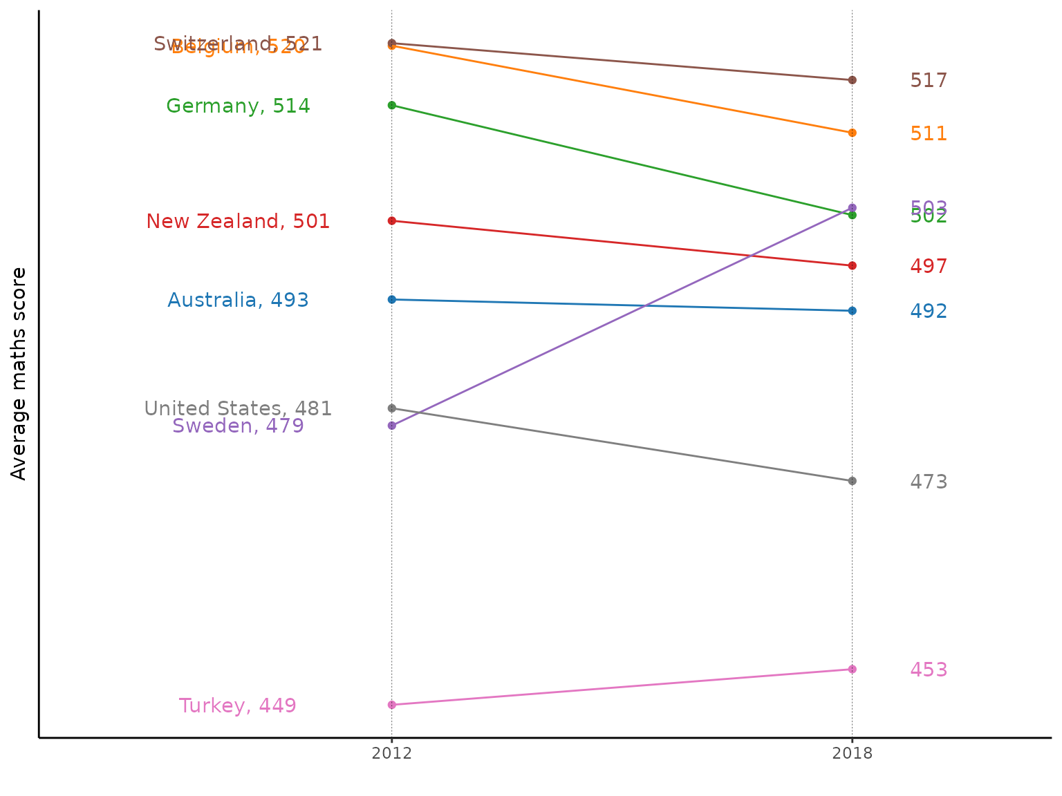
The figure above assists us in deducing the score change in the different countries from the year 2012 to 2018. This figure enables us to deduce that Albania, Qatar, and Peru have significantly boosted their average mathematics score between these years. While we also observe drop in average mathematics score for Japan.
Similarly, you may import student data for any chosen year and experiment with the PISA scores or additional analysis of these datasets with their other variables that assist contributor comprehend the data. Refer to our articles here for additional interesting analyses and plots.